The Engineering behind Figma’s Vector Networks

Adobe Illustrator introduced the pen tool back in 1987 as a tool for creating and modifying paths. Since then the pen tool has become incredibly widespread, so much so that is has become the de facto icon of the graphic design industry.
The pen tool’s functionality hasn’t changed significantly in the 30 years since its introduction. Just click and drag to create smooth curves. Designers have learned to work with it, and around its idiosyncrasies.

The pen tool
But Figma felt like they could improve some aspects of how the pen tool worked, so they had a go at redesigning it. Instead of it being used to work with traditional paths, they improved the pen tool by creating what they call Vector Networks.
In this post we will go through what Vector Networks are and what problems they try to solve. After we’ve defined what Vector Networks are, we will take a look at some of the engineering challenges you would face if you were to take a stab at implementing them.
This post can be thought of as an introduction to a really interesting problem space, and as a resource for people interesting in making use of some aspects of Vector Networks for future applications. I hope it succeeds in providing value to both developers being introduced to new concepts and ideas, and to designers interesting in learning more about the tool they know and love.
I will start off by laying out the core concepts behind the pen tool, and from there we will move onto Figma’s Vector Networks.
Paths
The pen tool is used to create and manipulate paths.
If you’ve every worked with graphics software like Illustrator before, you’ve worked with paths. Paths are a series of lines and curves that may or may not form a loop.

Some paths
The path to the left loops, while the path to the right doesn’t. Both of these are valid paths.
The main characteristic of paths is that they form a single continuous unbroken chain. This means that each node can only be connected to one or two other nodes.

Not valid paths
However, you could construct these shapes from multiple paths if you position them correctly together.

Multiple paths are used to create more complex shapes
From a combination of paths, you can create any shape imaginable.

This beer glass, for example, is just a combination of five different paths positioned and scaled a certain way.

The building blocks of paths
A path is made up of two things, points and lines.

Points and lines
The points are known as nodes (or vertices) and the lines are called edges.

Together, they make a path
Any path can be described as a list of nodes and edges.

This path can be described as the series of nodes (0, 1, 2, 3, 4). It could also be thought of as the series of the edges that composed it. That list of edges would be (0, 1), (1, 2), (2, 3), (3, 4), (4, 0).
You can think of this like the dot to dot puzzles that you used to do as a kid: Draw the edges of the path in the order that the points lay out.

But instead of a kid drawing lines between numbered points on a paper, a cold calculating machine does it along the cartesian coordinate system.

Edges
An edge is a connection between a pair of nodes. Visually, edges are a line from node a to node b.
But that line can be drawn in a lot of different ways. How do you describe those different types of lines?
Edges fall into two categories, straight and curvy.

Straight edges are as simple as they seem, just a line from a to b. But how are those curvy edges defined?
Bezier curves
Curvy edges are bezier curves. Bezier curves are a special type of curve defined by four points.

The positions of the two nodes in our edge make up the start and end points of the curve. Each of the two nodes has a control point.
In most applications, these control points are shown as handles that extend from their respective node. These handles are used to control the shape of the curve.
Bezier curves can be chained to make more complex shapes that a single curve can’t draw on its own. They can also be combined with straight lines to make some cool designs.

But what exactly are the handles doing? How do the handles tell the computer to draw the curve like it does?
Computers draw curves by splitting them into straight lines and drawing the individual lines.

The more lines you split a curve into, the smoother the curve becomes.

So to draw the curve we need to know how to get the different points that make up the curve. If we compute enough of them, we get a smooth curve.

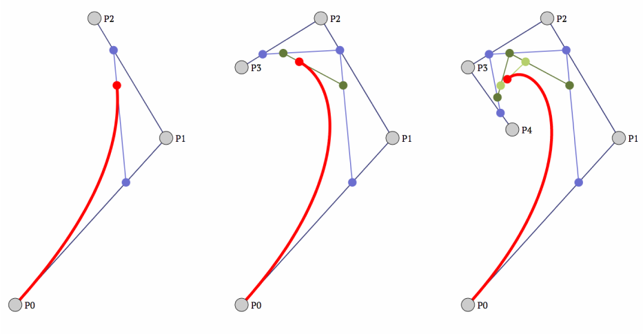
Computing a point on a bezier curve
Let’s compute the point at 25% point of the curve. We can start by connecting the control points with a third blue line.

Then for each blue line, we draw a blue dot at the 25% point of the line.

Next, draw two green lines between the three blue dots.

And we repeat the same step as we did with the blue dots. Draw green points at the 25% points of the green lines.

And then one more red line between the newly created green points.

Then we add a red point at the 25% point of the red line.

And just like that, we’ve computed the point at the 25% point of the curve.
From now on we’ll refer to points on curves through a t value, where t is a number from 0 to 1. In the above example, the point would be at t=0.25 (25%).

t=0.25, t=0.5 and t=0.75
This way of computing the point at t is called De Casteljau’s algorithm and can also be used to subdivide a bezier curve. Using the points we created along the way, we can also subdivide the bezier curve into two smaller bezier curves.

Bezier curves are pretty amazing things. Shaping the curve by adjusting the handles feels surprisingly natural, and chaining them together allows you to create detailed and complex shapes.

And for computers, they’re stable and inexpensive to compute. For this reason they’re used for everything from vector graphics to animation curves and automobile bodies.
You can see an interactive demo of bezier curves at Jason Davies’ site. It’s fascinating to watch a series of straight lines trace out a smooth curve.
From https://jasondavies.com/animated-bezier
The creative constraints of paths
Earlier in this post, paths were defined as a continuous series of lines and curves that may or may not form a loop.
The fact that paths are a single continuous chain is a pretty big limitation.
It means three way intersections are not possible using a single path. To create a three way intersection, two or more paths will have to be used. This means dealing with positioning and grouping different paths together. It also means that changes to a single path can lead to changes to multiple other paths.
But that’s simply the routine. Seasoned designers know how paths behave, they can plan around it without really thinking about it. For a static design it doesn’t really matter how many paths and layers you have to create if the piece is planned properly upfront.
But for some situations the constraints that paths impose cause a lot of friction.
Vector Networks
In 2016, Figma introduced Vector Networks. They lift the “single continuous” limitation by allowing any two nodes to be joined together without restrictions.
“A vector network improves on the path model by allowing lines and curves between any two points instead of requiring that they all join up to form a single chain.”

Source: https://www.figma.com/blog/introducing-vector-networks/
The cube is the quintessential example for demonstrating Vector Networks.

Via traditional paths, you would have to create at minimum 3 different paths to describe this shape.

This creates a lot of friction for a seemingly simple and common shape. To modify the cube, you would have to modify two or three different paths. But with Vector Networks you can simply grab an edge and move it around, and the shape behaves like you would expect.

So if you would want to increase the extrusion of the cube, you could just grab the two appropriate edges and move them together.

This is the big selling point for Figma’s Vector Networks. Ease of use.
Vector Networks don’t enable you to create something that you couldn’t create with other tools, but it does remove a lot of the friction in the process of creating things.
And you can take this even further. Say you want to add a hole to the side of the cube.

Just start off by selecting and copying the sides of the cube. You can then duplicate those edges and scale them to the size you want them to be.

And just like that, you have a cube with a hole.

And to make this hole believable, you just need the inner edge.

Again, Vector Networks may not allow you to create something you couldn’t otherwise. Instead, they enable workflows that weren’t previously possible.
Creating Vector Networks
With an understanding of what Vector Networks are, we can now take a look at how we would go about implementing them.
Graph
The main data structure behind Vector Networks is a graph. A graph can be thought of as a collection of nodes and edges.

A graph
Nodes
A graph may have any number of nodes. For our purposes nodes have two properties, a unique id and a position.

Edges
Edges are the connection between two nodes. Each edge is a composed of two edge parts. An edge part contains a node’s id and an optional control point.
The labels n0 and n1 will be used to refer to the nodes at the start and end of an edge, respectively. The control points will be labeled cp0 and cp1.

If the control points of the edge are omitted, the edge becomes a straight line.
Filling the holes
Source: https://www.figma.com/blog/introducing-vector-networks/
When working with vector networks, the Fill tool allows you to “toggle” the fill of different “areas” of the graph.

These areas can be defined as a sequence of node ids that go in a circle, a loop, if you will.
This loopy sequence is referred to as a cycle. In the above example, the cycle would consist of the nodes n0, n1, n3, n4, n5, n6 and n7. These cycles will be written like (0, 1, 3, 4, 5, 6, 7).
If you were to count the different visually distinct “areas” of the cycle your answer would probably be three, but you could easily find more than three cycles.

What makes this correct or incorrect?
The sequence (0, 1, 2, 3, 4, 5, 6, 7) is a cycle and it loops, but it is not what we’re looking for. The problem can be illustrated with the “how many triangles” puzzle you might have seen on Facebook.

How many triangles are in this image?
You should be able to count 24 different triangles depending on which areas you choose to include.

But that’s not what we want. What we need to find are the 16 small areas.

We need a way to find the “small cycles” in the graph.
Minimal cycle basis
This paper on Minimal Cycle Basis is a bit less dense than most others academic papers (and it has pictures!). Its goal is:
…to compute a minimal number of cycles that form a cycle basis for the graph.
What does “Minimal Cycle Basis” mean?
It’s just a fancy way to refer to all of the “small areas” of a graph. You can think of these as the “visually distinct” areas of a graph. Enclosed areas.
Left or right?
The main tool for finding the “minimal cycle basis” will be determining which edge to choose based on left- or rightness.

Should we go to a or b?
We’ll think of this in terms of clockwise and counter clockwise.

curr for current, prev for previous
When traveling left, we choose the counter clockwise most edge (CCW) relative to the previous one.

CCW
When traveling right, we choose the clockwise most edge (CW) relative to the previous one.

CW
The algorithm
We will be finding the minimal cycle basis for the graph we saw earlier.

The first step is choosing the leftmost node in the graph.

When traveling from the first node, we want to go clockwise (CW). But relative to which edge?
For the first node, we imagine that the previous edge is “below” the current one. We then pick the CW edge relative to that.

In this case a is more CW relative to prev than b, so we’ll walk to a.

After the first walk, we start picking the CCW edge.

In this case, that’s b. We repeat the previous step and keep selecting the CCW edge until we reach the original node.

When we reach the original node again, a cycle is found.

We now have the first small cycle in the graph.

When a cycle has been found, the first edge of the cycle is then removed from the graph.

The first edge, (n0 n1), is removed
Then, the filaments of the first two nodes in the cycle are removed.

In this case, we only have a single filament
Filaments are nodes that only have one adjacent edge. Think of these as dead ends. When a filament is found, we also check whether or not the single adjacent node is a filament. This ensures that the first node of the next cycle has two adjacent nodes. We’ll see an example of this later.
Now we pick the first node in the next cycle. In our graph, there are two equally left most nodes.

When this happens, we pick the bottom node, n1 in this case.

We then repeat the process from before. CW from the bottom for the first node, then CCW from the previous node until we find the first node.

We find the cycle (1, 2, 3).

Now we have the cycles (0, 1, 3, 4, 5, 6, 7) and (1, 2, 3).

Then we remove the first edge of the cycle and filaments like before. We start by removing the filaments connected to the first two nodes of the cycle.

We keep going until there aren’t any filaments left.

Finding the next cycle is pretty obvious.

CW then CCW
We now have all the cycles of the graph.

This is the minimal cycle basis of our graph! Now we can toggle the fills of these cycles as we please.

The math
I want to dig into how the clockwise-ness of an edge relative to another edge is determined.
The only prerequisite for understanding this section are vectors; arrows pointing from one point of a 2D coordinate system to another.

i = (1, 0), j = (0, 1)
With two vectors sitting at the origin, i and j, we can create a square like so.

For the unit vectors (1, 0) and (0, 1) the square has an area of 1.

We can do this with any two vectors.

This shape is called a parallelogram. Parallelograms have one property that we care about, which is that their area is equal to the absolute value of their determinant.
That may sound like jargon, but the determinant happens to be really useful for us. Take a look at what happens when we move the vectors of the one-by-one square closer together.

When the vectors get closer, their area gets smaller. And when the vectors are parallel, the determinant and area become 0.
At this point the natural question to ask is what happens when we keep going and the blue arrow is to the right of the green arrow?

The determinant becomes negative!
When the blue vector j is to the left of the green vector i the determinant of the parallelogram becomes negative. When the opposite is true it becomes positive.
The implication for our use case is that we can check whether the determinant of two vectors is positive or negative to determine whether or not a vector is to the left or right of another vector.
And we can do this no matter the direction because the area of a parallelogram does not change depending on the orientation of the vectors that create it.

The determinant changes when the orientation of the vectors change relative to each other.
With this knowledge as our weapon, we can create a function, det(i, j), that takes in two vectors and returns the determinant.

The function will return a positive value when j is to the left (CCW) of i.
Applying the math
Say we’re in the middle of the finding a cycle and we’re deciding whether or not to move to n0 or n1.

Let’s move this into the coordinate system.

We’ll start off with a.

We want to get the vector from curr to a, which we do by subtracting curr from a. We’ll call this new vector da.

We can do the same for curr using prev.

Now we can determine whether a is left of curr by computing the determinant of the parallelogram that da and dcurr form.

Note that the order is important. If we use da as i the area is negative. If we use it as j it becomes positive.

We can do the same with b.

With this information as our weapon, we know whether or not a, b and curr are left or right of each other.
What do we do with this information?
The green zone
We will be focusing on determining whether da is more CCW than db relative to curr. Simply put, is da left of db?
If da is more CCW than db relative to dcurr, da can be said to be better than db.
The first step is to determine whether the angle between dcurr and db is convex.

This “convexity” can more easily visualized by shifting dcurr back and imagining an arc like so:

The angle is convex
If the angle is convex, we we use the following expression to check whether da is better than db.

The ∨ symbol represents the logical OR operator in math.
Let’s take a look at the individual parts of this expression.

Is da CCW of dcurr?

Is da CCW of db?
I find that it’s pretty hard to visualize this mentally, so I think of the two different expressions creating a “green zone” where da is better than db.
For the first part of the expression (is da left of dcurr), the green area looks like so.

The second part of the expression asks if da is left of db. The green area look looks like so.

And since it’s an OR expression, either of these sub-expressions being true would result in a being better than b. Thus, the green area looks like this:

Is a better than b?
We use this to determine the better-ness of a when the angle is convex.
But what if the angle from dcurr to db is concave?

Then the expression looks like so:

The only thing that changed here is that the logical OR operator (∨) changed to the logical AND operator (∧).
Let’s take a look at what happens with the green zones using this expression.

Is da left of dcurr?

Is da left of db?
And since these sub-expressions are joined by logical AND, the green zone looks like so:

Using this method, we can always get the CCW or CW most node. And the great thing is that this method is independent of rotation and really cheap to compute.
Computing the determinant
Given two vectors, the determinant can be computed with this formula:

Intersections in the graph
Let’s go back to our graph for a bit.

This graph is the simplest, most optimistic case. This graph only has straight lines, and no two lines cross each other.

This box shape has an intersection. The edge (0, 2) crosses the edge (1, 3).

With the intersection, the above area looks fillable. But defining the “filled area” is pretty difficult.

What makes defining this area so difficult? Consider this rectangle and line.

There are two intersections with the edge (4, 5) intersecting (0, 1) and (2, 3).

Say the area left of the line is filled. What happens if we move the line left?

Obviously the area shrinks, but what if we keep going and move the line outside of the rectangle? Which of these outcomes below should be the result, and why?

In this case kinda feels like the rectangle should be empty. But what if we move the line right?

Should it then be filled? Sure, but what if we move the line up or down instead? Should the rectangle fill or empty when the line is no longer separating the two sections?
Expanding the graph
This is how I believe Figma solves this problem. I call it “expanding the graph”, but the engineers at Figma probably use a different vocabulary to describe it.
Expanding the graph means taking each intersection, creating a node at the point of the intersections, and then splitting the edges that intersected each other at that point.
This is the original graph:

The edge (0, 2) intersects the edge (1, 3). When expanded, the graph would look like so:

A new node, 5 would be added at the point of the intersection.
The edges (0, 2) and (1, 3) have been removed and replaced by the edges (0, 5), (5, 2), (1, 5), and (5, 3).

The structure of the graph has been changed
Here’s a graphic that should illustrate this a bit more clearly.

Expanding an intersection
Multiple intersections
These steps are pretty simple for line edges with a single intersections. But each edge can have multiple other edges intersecting it, and two cubic bezier curves can create 9 intersections.

This complicates things a bit. Let’s take a look at a bezier-line intersection.

The best way to go about this is to treat the intersections for an edge as separate from the edge that intersected it.

The t values go from 0 at the start of the curve to 1 at the end of it
The line has two intersections at t = 0.3 and t = 0.7. The bezier has two intersections, but at t = 0.25 and t = 0.75.
Before we move on with this example, I want to introduce a different way of thinking about edges since I believe it will help with the overall understanding of the problem.
Duplicate edges
Two nodes may be connected multiple times by different edges.

In this graph, an edge represented by the node pair (2, 3) could represent either of the two edges that connect n2 and n3.
To get around this problem, we will give each edge a unique id.

For most future examples, I will still refer to edges by the nodes they connect since I feel it’s easier to think about. But for the next example it’s better to separate nodes and edges.
Intersection map
We can structure the data for the intersections of the edges like so:

Creating nodes at the intersection points of edges
When we encounter an intersection, we create a node whose position is at the intersection. We then add intersections to an intersection map that will contain the intersections for each edge with a corresponding t value and a nodeId. These intersections are sorted by the t value.

For the intersection with the lowest t value, we create an edge with the first edge part having the nodeId of the first edge part of the original edge. The second edge part should contain the nodeId of the intersection. This creates the edge (2, 4).

Subsequent edges will have the first edge part’s nodeId be the nodeId of the previous intersection and the second nodeId be the nodeId of the current intersection. In this example, that edge is (4, 5).

One additional edge will be created for each edge with any intersections.
The first edge part’s nodeId will be the nodeId of the last intersection and the second edge part’s nodeId will be the nodeId of the second edge part of the original edge.
This was a bit of a mouthful, so hopefully this graphic helps a bit with understanding that alphabet soup.

Separating the intersections of an edge from the edges that created those intersections makes it easier to think about. It alleviates some of the complexity that might arise from multiple edges intersecting with each other.

Self-intersection
Cubic beziers can self-intersect.

This, unfortunately, means that every single cubic bezier edge has to be checked for self-intersection. It’s an interesting problem that involves finding the two different t values that the bezier intersects itself at, but I won’t be covering how to find those values here.
Once you have the t values, a self-intersecting bezier can be expanded like so:

The blue node should be invisible to the user
We insert n3 since having a node with an edge that has itself on both ends of the edge is problematic, but it should be hidden from the user.

Intersecting the loop of a self-intersecting bezier

Removing n3 at the first opportunity
Curvy edges
Earlier we covered the CW - CCW graph traversal algorithm to find the minimal cycle basis (small areas).

Finding the better (counter clockwise most) point adjacent to curr
But the algorithm described in the paper was designed to work with nodes connected by straight lines that don’t intersect. Introducing edges defined by cubic beziers introduces significant complexity.

Which edge to choose, blue or green?
In the example above, we can find out that the blue edge is better than the green one by using the determinant. We are stilling defining better to mean the CCW most edge.
When working with cubic bezier curves, the naive solution would be to just convert the bezier to a line defined by the points at the start and end of the curve.

But that idea breaks down as soon as one edge curves over the other.

Oops
Let’s take a fresh look at a bezier curves and try to work from there.

Looking at this, we notice that the tangent at the start of the curve, n0, is parallel to the line from n0 to cp0. So to get the direction at the start of the edge we can use the line (n0, cp0).
For clarity, the start of our edge, n0, is the same node as curr.

So by converting edges defined by cubic beziers into a line defined by (n0, cp0), we get the initial angle of the curve.

This seems like a good solution when looking at the “curve around” case.

Looks like we’ve solved the problem. Right?
No intersections
Before we move on to further edge cases, it helps to understand that any solutions assume that no two edges may intersect when deciding which edge to travel.

This is not allowed
The edges of the graph we’re traversing must not have any intersections when we compute the cycles (minimal cycle basis) of the graph.
We can only operate on an expanded graph.
Like we covered earlier, an expanded graph is a graph that has replaced all intersections with new nodes and edges. So if the original, user-defined graph has any intersections, they would have to be expanded before we can find the graph’s cycles.

The same edges as above, but expanded
Parallel edges
The next edge case is two edges being parallel (pointing in the same direction).

If the lines go in the same direction, determining which is better is impossible without more information.
Here are a few possible solutions for the cases where the control points of the curves are parallel.
Point at t
What if we just take the point on the curve at, for example, t = 0.1?

This produces the correct result for curves of a similar length, but we can easily break this with one curve being significantly bigger than the other.

This is effectively the same problem as the “curve around” case we saw earlier.
Point at length
Instead of taking a point at a fixed t value, we could take a point at some length along the curve. The length would be determined by some point on the smaller curve, e.g. at t=0.1.

I have not tried implementing this since I have another working solution, but this could possibly be a viable and performant solution if it works for all edge cases.
Lasers!
The next solution is a bit esoteric but produces the correct result. This is the solution I’m currently using.

We begin by splitting each bezier at t = 0.05 (image above is exaggerated). We then tesselate each part into n points.
Then, for each point of the tesselated bezier, we check whether a line from n0 to that point intersects the other edge.

It’s pretty hard to see what’s going on at this scale, so let’s zoom in a bit.

When a point intersects the other edge, we use the point before it.

Found an intersection
Let’s zoom in a bit.

The intersection close up
For the other edge, we have no intersection.

In that case, we just use the end of the edge as the direction line.

With this method we’ve produced lines that seem to represent their respective curves.

And this also works for the “curve around” case.

But it fails for a “curve behind” case.

This would produce the green edge as the more CCW edge, which is wrong.
My solution to this problem is to shoot an infinite laser in the direction of the previous edge.

We then check whether the points of the tesselated bezier intersect this laser.

But a line from n0 to the points would never intersect the laser.

Passes right through
Instead, we can create a line from the current point to the previous point and use that for the intersection test.

When we intersect the laser, we use the previous point. The previous point will always be on the correct side of the laser.

The point we use
And like that, we have a solution.

Parallel, but in reverse!
It could also be the case that the blue or green edges, a and b respectively, could be parallel to the edge from curr to prev.

a is parallel to prev
The process for finding the better edge follows a process similar to the one described above so we will cover this very quickly.
There are two cases:
A or B are parallel to Prev , but not both
If either a or b, but not both, are parallel to prev, we can simply compare the parallel edge to prev.
If the parallel edge is CW of prev, the parallel edge is better.
If the parallel edge is CCW of prev, the other edge is better.
Think a bit about why this is true.
If one edge is parallel to prev and curves CW, and the other is not parallel to prev, then the parallel edge is as CCW as can be. This means that the green zone for the other edge is completely empty.
The reverse is true if the parallel edge curves CCW, since it would be as CW as possible. This means that the green zone for the other edge is the whole circle.

Both A and B are parallel to Prev
Using the same laser solution as before, this case is covered.
Cycles inside of cycles
Now we’re going to look at fills for a bit.
Let’s take a look at a basic example of a graph with a cycle inside of another cycle.

You would expect the graph’s areas to be defined like so:

But as it stands, if you hover over the outer area you get a different, unsatisfactory result.

But this makes sense. Let’s take a look at the nodes of the graph.

The cycle (0, 1, 2, 3) describes the outer boundary of the area we want, but we aren’t describing the “inner boundary” of the area yet.
Let’s take a look at how we can do that.
Even-odd rule
Telling a computer to draw the outline of a 2D shape is simple enough. But if you want to fill that shape, how do you tell the computer what is “inside” and what is “outside”?

One way of finding out whether a point is inside a shape or not is by shooting an infinite laser in any direction from that point and counting how many “walls” it passes through.
If the laser intersects an odd number of walls, it’s inside of the shape. Otherwise it is outside of the shape.

Intersects 1 wall, we’re inside of the shape

Intersects 4 walls, we’re outside of the shape
This works for any 2D shape, no matter which point you choose and which direction you shoot the laser in.
This also helps in the case of nested paths.

This gives us an idea for how we can define the “inner boundary” of a shape.

Reducing closed walks
Let’s look at a graph with a cycle nested inside of another cycle, but with an edge connecting two nodes of the cycles.

This will lead back to how we can think about nested cycles and give us a deeper understanding on how to think about them.
Let’s find the cycles. We use the same CW-CCW method as usual.

With this method, we go on what looks like a small detour around the inner cycle.

When we reach the node we started at, this is what the cycle looks like.

This is the first cycle we’ve seen where we cross a node twice (both n3 and n4). Something interesting appears when we take a look at the direction that the cycle takes throughout the graph.

We start off traveling CCW, but when we cross the edge from the outer cycle to the inner cycle the orientation we travel seems to flip.
I will state for now that we want to separate the outer cycle from the inner cycle and treat the edge between them as if it didn’t exist. I will go into the why later and explain the how here.

We take all repeated nodes, in this case n3, and remove them from the cycle. We also remove any nodes that are between the two repeated nodes.
You might notice that n4 is also repeated, but since it’s “inside” of the part of the cycle that n3 removes, we can ignore it.
We leave one instance of the repeated node, and then we have the cycle that would have been found if the crossing didn’t exist.

We then mark the edge that connected the outer cycle from the inner cycle. I call these marked edges crossings.

It could also be the case that an outer-inner cycle combo has multiple crossings.

In that case, we mark all edges adjacent to the node connected to the outer cycle as a crossing.

And after all this is done, our cycles look like so:

Subcycles
Instead of referring to “inner” and “outer” cycles, I will refer to subcycles and parent cycles. This will make it easier to think about multiple cycles relative to each other.
Having said that, let’s introduce a third cycle.

When we hover over the outermost cycle, what do you expect to happen?

Because of the even-odd rule, the innermost cycle is filled too!

To fix this, we can introduce the concept of direct subcycles.

Parent cycles (blue) and their direct subcycles (green)
A parent cycle may have multiple direct subcycles. But due to the non-intersection rule, a subcycle may only have a single parent cycle.
Let’s take a look at how this works.

This graph has a a rectangle, our outermost cycle, which has two direct subcycles: a diamond and an hourglass. The diamond has two direct subcycles of its own, and the hourglass has three direct subcycles.
We will begin with the rectangle and its direct subcycles. We will name them, c0, c1 and c2.

The user has decided to fill some of these cycles, and leave some of them empty.

c0 and c1 are filled, and c2 is empty
Let’s draw the graph without a stroke and with a gray fill. When drawing this graph we start with the outermost cycle, c0.

The graph to the left with the render to the right
Since c0 is filled, we draw it. If it were not filled we could skip drawing it. We can shoot a laser out of the rectangle and see that it intersects the walls of the rectangle once, so we can expect it to be filled considering the even-odd rule.

This may seem really obvious, but it’s good to have the rules of the game laid out clearly before we move on.
Next we want to draw c1, the diamond in our graph. It was filled, just like the rectangle so we should draw it as well. But if we try to draw the diamond as well, we get the wrong result.

Our laser is intersecting two walls as a result of drawing both of the shapes when the have the same fill setting.

We intersect an even number of walls, so we’re “outside” of the shape
So to draw the image the user wanted we can simply skip drawing the diamond since the parent cycle implicitly draws direct subcycles with the same fill setting.
The hourglass, c2, is supposed to be empty. With that being the case, just not drawing it seems like a reasonable conclusion. But since the parent cycle (rectangle) has already drawn the hourglass as if it were filled we need to “flip” the fill by drawing the hourglass.

And again, if we try to use the laser intersection method we see that the number of intersections is 2, an even number. And with the even-odd rule, an even number of walls means you’re “outside” of the shape.

Now that we’ve drawn the rectangle and its direct subcycles, we can move onto the direct subcycles of those.

When working with c3 and c4, the direct subcycles of c1, we can treat them as if they’re direct subcycles of c0 since c1 had the same fill setting.
For c3, we want to “flip” the fill setting so we draw it. But c4 has the same fill setting as its parent cycle so we don’t draw it.

Even number of intersections so we’re outside of the shape
And we can think of c5, c6 and c7 in the same way. We don’t care whether they’re filled or empty when rendering them. We care whether or not they have the same fill as their parent cycle.
We only need to draw cycles if their parent cycle has the opposite “fill setting” as themselves. If they have the same fill setting, we don’t have to draw them.

This means that when drawing cycles, start by drawing the outermost “filled” cycle and then look at that cycle’s subcycles. If a subcycle has the same fill setting as its parent cycle, it should not be drawn.

Contiguous cycles
A graph may have multiple “clusters” of cycles.

I use the phrase contiguous cycles to describe the “togetherness” of the cycles, if you will. I often think of these contiguous groups of cycles as being in different colors.

Finding these contiguous cycles can be done with a depth-first traversal:

Start at the first node of the cycle

Color each node you find
But remember the crossings? In the search, you may not crawl to adjacent nodes by edges marked as crossings.

So in the end, our colors actually look like this:

Take this group of contiguous cycles nested inside another group of contiguous cycles:

Because of the non-intersection rule we know that if one of the nodes in a group of contiguous cycles is inside of a cycle not in the group, all of them are.

This “contiguous cycles” idea is maybe not the most interesting part of this post on the surface, but I’ve found it to be useful when working on Vector Networks.
Partial expansion
When hovering an area defined by intersections, we are showing a cycle of the expanded graph.
Take this triangle as an example.

If we hover over one of its areas, we see an area defined by nodes that don’t exist yet.

What the blue striped area represents is the area whose fill state would be “toggled” if the user clicks the left mouse button. This area does not exist on the graph as the user defined it. It exists as a cycle on the expanded version of the original graph.

The expanded graph
When the user clicks to toggle the fill state of the area, we would first have to expand the graph for the nodes and edges that make up that area to exist.

The expanded graph
But by doing that we’ve expanded two intersections that we didn’t need to expand to be able to describe the area. These expansions are destructive in nature and should be avoided when possible.
Instead, we can partially expand the graph by only expanding the intersections that define the selected cycle.

Partially expanded graph
This allows us to maintain as much of the original graph as possible while still being able to define the fill.
Implementing partial expansions
The basic implementation is reasonably simple. When you create the expanded graph, just add a little metadata to each expanded node that tells you which two edges of the original graph were used to create it and at what t values those intersections occurred.
Then when the cycle is clicked, iterate over each node. If the node exists in the expanded graph but not the original graph, add it to a new partially expanded graph.
There are edge cases, but I will not be covering them here.
Omitted topics
Here are some of the topics that I decided to omit for this post. Go have a stab at them yourself!
Joins
Figma offers three types of joins. Round, pointy and square. How could these different types of joins be implemented?

Stroke align
Figma also offers three ways to align the stroke of a graph: center, inside and outside.
How do you determine inside- or outside-ness and what happens when the graph has no cycles?
Boolean operations
Figma, like most vector graphics tools, offers boolean operations. How could those be implemented?
Paper.js is open source and has boolean operations for paths, maybe you can start there?
Future topics
These are some of the more open-ended features and ideas I want to explore in the future.
A different way of working with fills
There are alternatives to how Figma allows the user to work with fills.
One possible solution I’m interested in exploring is multiple different “fill layers” that use one vector object as a reference. This would solve the “one graph, multiple colors” problem without having to duplicate the layer and keep multiple vector objects in sync if you want to make changes later on.
Animating the graph
Given an expression and reference based system similar to After Effects, what could you achieve when you combine it with Vector Networks?
Or maybe we could make use of a node editor similar to Blender’s shader editor or Fusion’s node based workflow?
There’s a lot of exploration to be done here and I’m really excited to dive into this topic.
In closing
Thanks for reading this post! I hope it served as a good introduction to what I think is a really interesting problem space. I’ve been working on this problem alongside school and work for a good while. It’s part of an animation editor plus runtime for the web I’m working on. I intend for a modified version of Vector Networks to be the core of a few features.
I’ve been working on implementing Vector Networks for a bit over half a year now. The vector editor is pretty robust when it comes to creating, modifying and expanding the graph. But the edge cases when modifying the fill state have been stumping me for quite a while now.
I wanted to have a fully working demo before publishing this post, but it’s going to be a few months until it’s stable enough for it to be usable for people that are not me.
The big idea behind the project is to be a piece of animation software that’s tailor-made for creating and running dynamic animations on the web. I’ll share more about this project at a later date.
I also just think that Figma’s Vector Networks are super cool and it’s really hard to find material about it online. I hope this post helps fix the lack of information that I encountered when attempting to find information about Vector Networks.
To be notified of new posts, subscribe to my mailing list.