A flowing WebGL gradient, deconstructed
A few weeks ago I embarked on a journey to create a flowing gradient effect — here’s what I ended up making:
Loading canvas...
This effect is written in a WebGL shader using noise functions and some clever math.
In this post, I’ll break it down step by step. You need no prior knowledge of WebGL or shaders — we’ll start by building a mental model for writing shaders and then recreate the effect from scratch.
We’ll cover a lot in this post: writing shaders, interpolation, color mapping, gradient noise, and more. I’ll help you develop an intuition for these concepts using dozens of visual (and interactive!) explanations.
If you just want to see the final code, I’ll include a link to the shader code at the end of the post (this blog is open source so you can just take a look).
Let’s get started!
Color as a function of position
Building the gradient effect will boil down to writing a function that takes in a pixel position and returns a color value:
type Position = { x: number, y: number };function pixelColor({ x, y }: Position): Color;
For every pixel on the canvas, we’ll invoke the color function with the pixel’s position to calculate its color. A canvas frame might be rendered like so:
for (let x = 0; x < canvas.width; x++) {for (let y = 0; y < canvas.height; y++) {const color = pixelColor({ x, y });canvas.drawPixel({ x, y }, color);}}
To start, let’s write a color function that produces a linear gradient like so:
Loading canvas...
To produce this red-to-blue gradient we’ll blend red and blue with a blend factor that increases from
function pixelColor({ x, y }: Position): Color {const t = x / (canvas.width - 1);}
Having calculated the blending factor
const red = color("#ff0000");const blue = color("#0000ff");function pixelColor({ x, y }: Position): Color {const t = x / (canvas.width - 1);return mix(red, blue, t);}
The mix function is an interpolation function that linearly interpolates between the two input colors using a blend factor between
A mix function for two numbers can be implemented like so:
function mix(a: number, b: number, t: number) {return a * (1 - t) + b * t;}
The mix function is often called “lerp” — short for linear interpolation.
A mix function for two colors works the same way, except we mix the color components. To mix two RGB colors, for example, we’d mix the red, green, and blue channels.
function mix(a: Color, b: Color, t: number) {return new Color(a.r * (1 - t) + b.r * t,a.g * (1 - t) + b.g * t,a.b * (1 - t) + b.b * t,);}
Anyway, mix(red, blue, t) produces a red-to-blue gradient over the width of the canvas (the
Loading canvas...
When x == 0 we get a x == canvas.width - 1 we get a
If we want an oscillating gradient (red to blue to red again, repeating), we can do that by using sin(x) to calculate the blending factor:
function pixelColor({ x, y }: Position): Color {let t = sin(x);t = (t + 1) / 2; // Normalizereturn mix(red, blue, t);}
Note: sin returns a value between mix function accepts a value between
This produces the following effect:
Loading canvas...
Those waves are very thin! That’s because we’re oscillating between red and blue every
We can control the rate of oscillation by defining a frequency multiplier. It will determine over how many pixels the gradient oscillates from red to blue and red again. To produce a wavelength of
const L = 40;const frequency = (2 * PI) / L;function pixelColor({ x, y }: Position): Color {let t = sin(x * frequency);// ...}
This produces an oscillating gradient with the desired wavelength — try changing the value of
Loading canvas...
Adding motion
So far we’ve only produced static images. To introduce motion, we’ll update our color function to take in a time value as well.
function pixelColor({ x, y }: Position, time: number): Color;
We’ll define time as the elapsed time, measured in seconds.
By adding time to the pixel’s
let t = sin((x + time) * frequency);
But scrolling one pixel a second is very slow. Let’s add a speed constant time by it:
const S = 20;let t = sin((x + time * S) * frequency);
Here’s the result — try adjusting the speed via the
Loading canvas...
Voila, we’ve got movement!
These two inputs — time and the pixel’s position — will be the main components that drive our final effect.
We’ll spend the rest of the post writing a color function that will calculate a color for every pixel — with the pixel’s position and time as the function’s inputs. Together, the colors of each pixel constitute a single frame of animation.
Loading canvas...
But consider the amount of work that needs to be done. A
WebGL shaders run on the GPU, which is useful to us because the GPU is designed for highly parallel computation. A GPU can invoke our color function thousands of times in parallel, making the task of rendering a single frame a breeze.
Conceptually, nothing changes. We’re still going to be writing a single color function that takes a position and time value and returns a color. But instead of writing it in JavaScript and running it on the CPU, we’ll write it in GLSL and run it on the GPU.
WebGL and GLSL
WebGL can be thought of as a subset of OpenGL, which is a cross-platform API for graphics rendering. WebGL is based on OpenGL ES — an OpenGL spec for embedded systems (like mobile devices).
Here’s a page listing the differences between OpenGL and WebGL. We won’t encounter those differences in this post.
OpenGL shaders are written in GLSL, which stands for OpenGL Shading Language. It’s a strongly typed language with a C-like syntax.
There are two types of shaders, vertex shaders and fragment shaders, which serve different purposes. Our color function will run in a fragment shader (sometimes referred to as a “pixel shader”). That’s where we’ll spend most of our time.
There’s tons of boilerplate code involved in setting up a WebGL rendering pipeline. I’ll mostly omit it so that we can stay focused on our main goal, which is creating a cool gradient effect.
Throughout this post, I’ll link to resources I found helpful in learning about how to set up and work with WebGL.
Writing a fragment shader
Here’s a WebGL fragment shader that sets every pixel to the same color.
void main() {vec4 color = vec4(0.7, 0.1, 0.4, 1.0);gl_FragColor = color;}
WebGL fragment shaders have a main function that is invoked once for each pixel. The main function sets the value of gl_FragColor — a special variable that specifies the color of the pixel.
We can think of main as the entry point of our color function and gl_FragColor as its return value.
WebGL colors are represented through vectors with 3 or 4 components: vec3 for RGB and vec4 for RGBA colors. The first three components (RGB) are the red, green, and blue components. For 4D vectors, the fourth component is the alpha component of the color — its opacity.
vec3 red = vec3(1.0, 0.0, 0.0);vec3 blue = vec3(0.0, 0.0, 1.0);vec3 white = vec3(1.0, 1.0, 1.0);vec4 semi_transparent_green = vec4(0.0, 1.0, 0.0, 0.5);
WebGL colors use a fractional representation, where each components is a value between
void main() {vec4 color = vec4(0.7, 0.1, 0.4, 1.0);gl_FragColor = color;}
We can trivially convert the fractional GLSL color vec3(0.7, 0.1, 0.4) to the percentage-based CSS color rgb(70%, 10%, 40%). We can also multiply the fraction by 255 to get the unsigned integer representation rgb(178, 25, 102).
Anyway, if we run the shader we see that every pixel is set to that color:
Loading canvas...
Let’s create a linear gradient that fades to another color over the rgb(229, 154, 25) — it corresponds to vec3(0.9, 0.6, 0.1) in GLSL.
vec3 color_1 = vec3(0.7, 0.1, 0.4);vec3 color_2 = vec3(0.9, 0.6, 0.1);
I’ve been using this tool to convert from hex to GLSL colors, and vice versa
To gradually transition from color_1 to color_2 over the gl_FragCoord:
float y = gl_FragCoord.y;
float corresponds to a 32-bit floating point number. We’ll only use the float and int number types in this post, both of which are 32-bit.
Similar to before, we’ll use the pixel’s
const float CANVAS_WIDTH = 150.0;float y = gl_FragCoord.y;float t = y / (CANVAS_WIDTH - 1.0);
Note: I’ve configured the coordinates such that gl_FragCoord is (0.0, 0.0) at the lower-left corner and (CANVAS_WIDTH - 1, CANVAS_HEIGHT - 1) at the upper right corner. This will stay consistent throughout the post.
We’ll mix the two colors with GLSL’s built-in mix function.
vec3 color = mix(color_1, color_2, t);
GLSL has a bunch of built-in math functions such as sin, clamp, and pow.
We’ll assign our newly calculated color to gl_FragColor:
vec3 color = mix(color_1, color_2, t);gl_FragColor = color;
But wait — we get a compile-time error.
ERROR: ‘assign’ : cannot convert from ‘3-component vector of float’ to ‘FragColor 4-component vector of float’
This error is a bit obtuse, but it’s telling us that we can’t assign our vec3 color to gl_FragColor because gl_FragColor is of type vec4.
In other words, we need to add an alpha component to color before passing it to gl_FragColor. We can do that like so:
vec3 color = mix(color_1, color_2, t);gl_FragColor = vec4(color, 1.0);
This gives us a linear gradient!
Loading canvas...
Vector constructors
You may have raised an eyebrow at the vec4(color, 1.0) expression above — it’s equivalent to vec4(vec3(...), 1.0), which is perfectly valid in GLSL!
When passing a vector to a vector constructor, the components of the input vector are read left-to-right — similar to JavaScript’s spread syntax.
vec3 a;// this:vec4 foo = vec4(a.x, a.y, a.z, 1.0);// is equivalent to this:vec4 foo = vec4(a, 1.0);
You can combine number and vector inputs in any way you see fit as long as the total number of values passed to the vector constructor is correct:
vec4(1.0 vec2(2.0, 3.0), 4.0); // OKvec4(vec2(1.0, 2.0), vec2(3.0, 4.0)); // OKvec4(vec2(1.0, 2.0), 3.0); // Error, not enough components
Coloring areas different colors
Let’s color the bottom half of our canvas white, like so:
Loading canvas...
To do that, we’ll first calculate the
const float MID_Y = CANVAS_HEIGHT * 0.5;
We can then determine the pixel’s signed distance from the line through subtraction:
float y = gl_FragCoord.y;float dist = MID_Y - y;
What determines whether our pixel should be white or not is whether it’s below the line, which we can determine by reading the sign of the distance via the sign function. The sign function returns
float dist = MID_Y - y;sign(dist); // -1.0 or 1.0
We can calculate an alpha (blend) value by normalizing the sign to
float alpha = (sign(dist) + 1.0) / 2.0;
Blending color and white using alpha colors the bottom half of the canvas white:
color = mix(color, white, alpha);
Loading canvas...
Here, alpha represents how white our pixel is. If alpha == 1.0 the pixel is colored white, but if alpha == 0.0 the original value of color is retained.
Calculating an alpha value by normalizing the sign and passing that to the mix function may seem overly roundabout. Couldn’t you just use an if statement?
if (sign(dist) == 1.0) {color = white;}
You could, but only if you want to pick 100% of either color. As we extend this to smoothly blend between the colors, using conditionals won’t work.
As an additional point, you generally want to avoid branching (if-else statements) in code that runs on the GPU. There are nuances to the performance of branches in shader code, but branchless code is usually preferable. In our case, calculating the alpha and running the mix function boils down to sequential math instructions that GPUs excel at.
Drawing arbitrary curves
We’re currently coloring everything under MID_Y white, but the line doesn’t need to be determined by a constant — we can calculate the dist:
float curve_y = <some expression>;float dist = curve_y - y;
That allows us to draw the area under any curve white. Let’s, for example, define the curve as a slanted line
where
const float Y = 0.4 * CANVAS_HEIGHT;const float I = 0.2;float x = gl_FragCoord.x;float curve_y = Y + x * I;
This produces the slanted line in the canvas below — you can vary
Loading canvas...
We could also draw a parabola like so:
// Adjust x=0 to be in the middle of the canvasfloat x = gl_FragCoord.x - CANVAS_WIDTH / 2.0;float curve_y = Y + pow(x, 2.0) / 40.0;
Loading canvas...
The point is that we can define the curve however we want.
Producing an animated wave
To draw a sine wave, we can define the curve as:
where
const float Y = 0.5 * CANVAS_HEIGHT;const float A = 15.0;const float L = 75.0;const float frequency = (2.0 * PI) / L;float curve_y = Y + sin(x * frequency) * A;
This draws a sine wave:
Loading canvas...
At the moment, things are completely static. For our shader to produce any motion we’ll need to introduce a time variable. We can do that using uniforms.
uniform float u_time;
You can think of uniforms as per-draw call constants — global variables that the shader has read-only access to. The actual values of uniforms are controlled on the JavaScript side.
Within a given draw call, each shader invocation will have uniforms set to the same values. This is what the name “uniform” refers to — the values of uniforms are uniform across shader invocations within a given draw call. The JavaScript side can, however, change the values of uniforms between draw calls.
Uniforms are constant within draw calls but they are not compile-time constant, meaning you cannot use the value of a uniform in const variables.
Uniform variables can be of many types, such as floats, vectors, and textures (we’ll cover textures later). But what’s up with the u_ prefix?
uniform float u_time;
Prefixing uniform names with u_ is a GLSL convention. You won’t encounter compiler errors if you don’t, but prefixing uniform names with u_ is a very established pattern.
Note: There are similar conventions for the names of attributes and varyings (they’re prefixed with a_ and v_, respectively), but we won’t use attributes or varyings in this post.
Anyway, with u_time now accessible in our shader we can start producing motion. As a refresher, we’re currently calculating our curve’s
float curve_y = Y + sin(x * W) * A;
Adding u_time to the pixel’s
float curve_y = Y + sin((x + u_time) * W) * A;
But moving one pixel a second is quite slow (u_time is measured in seconds), so we’ll add a speed constant
const float S = 25.0;float curve_y = Y + sin((x + u_time * S) * W) * A;
Try varying
Loading canvas...
Applying a gradient to the lower half
Instead of the lower half being a flat white color, let’s make it a gradient (like the upper half).
The upper half’s gradient is currently composed of two colors: color_1 and color_2. Let’s rename those to upper_color_1 and upper_color_2:
vec3 upper_color_1 = vec3(0.7, 0.1, 0.4);vec3 upper_color_2 = vec3(0.9, 0.6, 0.1);
For the lower half’s gradient, we’ll introduce two new colors: lower_color_1 and lower_color_2.
vec3 lower_color_1 = vec3(1.0, 0.7, 0.5);vec3 lower_color_2 = vec3(1.0, 1.0, 0.9);
We’ll calculate a
float t = y / (CANVAS_HEIGHT - 1.0);vec3 upper_color = mix(upper_color_1, upper_color_2, t);vec3 lower_color = mix(lower_color_1, lower_color_2, t);
With this, we’ve effectively calculated two gradients. We’ll then determine which gradient to use for the current pixel’s color using alpha:
float alpha = (sign(curve_y - y) + 1.0) / 2.0;vec3 color = mix(upper_color, lower_color, alpha);
This applies the gradients to the halves:
Loading canvas...
Since the value of alpha is calculated using the sign of the distance, its value will abruptly change from
Let’s look at how we can make the split smoother using blur.
Adding blur
Take another look at the final animation and consider the role that blur plays:
Loading canvas...
The blur isn’t applied uniformly over the wave — a variable amount of blur is applied to different parts of the wave, and the amount fluctuates over time.
How might we achieve that?
Gaussian blur
When thinking about how I’d approach the blur problem, my first thought was to use Gaussian blur. I figured I’d determine the amount of blur to apply via a noise function and then sample neighboring pixels according to the blur amount.
That’s a valid approach — progressive blur in WebGL is feasible — but in order to get a decent blur we’d need to sample lots of neighboring pixels, and the amount of pixels to sample only increases as the blur radius gets larger. The final effect requires a very large blur radius, so that becomes incredibly expensive very quickly.
Additionally, for us to be able to sample the alpha values of neighboring pixels with any reasonable performance, we’d need to calculate their alpha values up front. To do that we’d need to pre-render the alpha channel into a texture for us to sample, which would require setting up another shader and render pass. Not a huge deal, but it would add complexity.
I opted to take a different approach that doesn’t require sampling neighboring pixels. Let’s take a look.
Calculate blur using signed distance
Here’s how we’re currently calculating alpha:
float dist = curve_y - y;float alpha = (sign(dist) + 1.0) / 2.0;
By taking the sign of our distance, we always get an opacity of 0% or 100% — either fully transparent or completely opaque. Let’s instead make alpha gradually transition from
const float BLUR_AMOUNT = 50.0;
We’ll change the calculation for alpha to just be dist / BLUR_AMOUNT.
float alpha = dist / BLUR_AMOUNT;
When dist == 0.0, the alpha will be dist approaches BLUR_AMOUNT the alpha approaches alpha to transition from
- when
distexceedsBLUR_AMOUNTthe alpha will exceed, and - the alpha becomes negative when
distis negative.
Both of those would cause problems (alpha values should only range from alpha to the range clamp function:
float alpha = dist / BLUR_AMOUNT;alpha = clamp(alpha, 0.0, 1.0);
This produces a blur effect, but we can observe the wave “shifting down” as the blur increases — try varying the amount of blur using the slider:
Loading canvas...
We can fix the downshift by starting alpha at
float alpha = 0.5 + dist / BLUR_AMOUNT;alpha = clamp(alpha, 0.0, 1.0);
Starting at alpha to transition from dist ranges from -BLUR_AMOUNT / 2 to BLUR_AMOUNT / 2, which keeps the wave centered:
Loading canvas...
Let’s now make blur gradually increase from left to right. To gradually increase the blur, we can linearly interpolate from no blur to BLUR_AMOUNT over the
float t = gl_FragCoord.x / (CANVAS_WIDTH - 1)float blur_amount = mix(1.0, BLUR_AMOUNT, t);
Using blur_amount to calculate the alpha, we get a gradually increasing blur:
float alpha = dist / blur_amount;alpha = clamp(alpha, 0.0, 1.0);
Loading canvas...
This forms the basis for how we’ll produce the blur in the final effect.
The blur currently looks a bit “raw”, but let’s put that aside for the time being. We’ll make it look awesome later in the post.
Let’s now work on creating a natural-looking wave.
Stacking sine waves
I often reach for stacked sine waves when I need a simple and natural wave-like noise function. Here’s an example of a wave created using stacked sine waves:
Loading canvas...
The idea is to sum the output of multiple sine waves with different wavelengths, amplitudes, and phase speeds.
Take the following pure sine waves:
Loading canvas...
If you combine them into a single wave, you get an interesting final wave:
Loading canvas...
The equation for the individual sine waves is
where
determines the wavelength, determines the phase evolution speed, and determines the amplitude of the wave.
The final wave can be described as the sum of
Which put into code, looks like so:
float sum = 0.0;sum += sin(x * L1 + u_time * S1) * A1;sum += sin(x * L2 + u_time * S2) * A2;sum += sin(x * L3 + u_time * S3) * A3;...return sum;
The problem, then, is finding
In finding those values, I first create a “baseline wave” with the
const float L = 0.015;const float S = 0.6;const float A = 32.0;float sum = sin(x * L + u_time * S) * A;
They produce the following wave:
Loading canvas...
This wave has the rough shape of what I want the final wave to look like, so these values serve as a good baseline.
I then add more sine waves that use the baseline
float sum = 0.0;sum += sin(x * (L / 1.000) + u_time * 0.90 * S) * A * 0.64;sum += sin(x * (L / 1.153) + u_time * 1.15 * S) * A * 0.40;sum += sin(x * (L / 1.622) + u_time * -0.75 * S) * A * 0.48;sum += sin(x * (L / 1.871) + u_time * 0.65 * S) * A * 0.43;sum += sin(x * (L / 2.013) + u_time * -1.05 * S) * A * 0.32;
Observe how
These five sine waves give us a reasonably natural-looking final wave:
Loading canvas...
Because all of the sine waves are defined by
Loading canvas...
We won’t actually make use of stacked sine waves in our final effect. We will, however, use the idea of stacking waves of different scales and speeds.
Simplex noise
Simplex noise is a family of
The dimensionality of a simplex noise function refers to how many numeric input values the function takes (the 2D simplex noise function takes two numeric arguments, the 3D function takes three). All simplex noise functions return a single numeric value between
2D simplex noise is frequently used, for example, to procedurally generate terrain in video games. Here’s an example texture created using 2D simplex noise that could be used as a height map:
Loading canvas...
It is generated by calculating the lightness of each pixel using the output of the 2D simplex noise function with the pixel’s
const float L = 0.02;float x = gl_FragCoord.x * L;float y = gl_FragCoord.y * L;float lightness = (simplex_noise(x, y) + 1.0) / 2.0;gl_FragColor = vec4(vec3(lightness), 1.0);
Note: The simplex_noise implementation I’m using can be found in this GitHub repository.
Loading canvas...
We’ll use 2D simplex noise to create an animated 1D wave. The idea behind that may not be very obvious, so let’s see how it works.
1D animation using 2D noise
Consider the following points:
Loading 3D scene
The points are arranged in a grid configuration on the simplex_noise(x, z):
for (const point of points) {const { x, z } = point;point.y = simplex_noise(x, z);}
By doing this we’ve effectively created a 3D surface from a 2D input (the
Fair enough, but how does that relate to generating an animated wave?
Consider what happens if we use time as the
Loading 3D scene
Putting this into code for our 2D canvas is fairly simple:
uniform float u_time;const float L = 0.0015;const float S = 0.12;const float A = 40.0;float x = gl_FragCoord.x;float curve_y = MID_Y + simplex_noise(x * L, u_time * S) * A;
This gives us a smooth animated wave:
Loading canvas...
A single simplex noise function call already produces a very natural-looking wave!
The same three
We scale
Lastly, we scale the output of the
Simplex noise returns a value between
Even though the simplex wave feels natural, I find the peaks and valleys to look too evenly spaced and predictable.
That’s where stacking comes in. We can stack simplex waves of various lengths and speeds to get a more interesting final wave. I tweaked the constants and added a few increasingly large waves — some slower and some faster. Here’s what I ended up with:
const float L = 0.0018;const float S = 0.04;const float A = 40.0;float noise = 0.0;noise += simplex_noise(x * (L / 1.00), u_time * S * 1.00)) * A * 0.85;noise += simplex_noise(x * (L / 1.30), u_time * S * 1.26)) * A * 1.15;noise += simplex_noise(x * (L / 1.86), u_time * S * 1.09)) * A * 0.60;noise += simplex_noise(x * (L / 3.25), u_time * S * 0.89)) * A * 0.40;
This produces a wave that feels natural, yet visually interesting.
Loading canvas...
Looks awesome, but there is one component I feel is missing, which is directional flow. The wave is too “still”, which makes it feel a bit artificial.
To make the wave flow left, we can add u_time to the x component, scaled by a constant
const float F = 0.043;float noise = 0.0;noise += simplex_noise(x * (L / 1.00) + F * u_time, ...) * ...;noise += simplex_noise(x * (L / 1.30) + F * u_time, ...) * ...;noise += simplex_noise(x * (L / 1.86) + F * u_time, ...) * ...;noise += simplex_noise(x * (L / 3.25) + F * u_time, ...) * ...;
This adds a subtle flow to the wave. Try changing the amount of flow to feel the difference it makes:
Loading canvas...
The amount of flow may feel subtle, but that’s intentional. If the flow is easily noticeable, there’s too much of it.
I think we’ve got a good-looking wave. Let’s move on to the next step.
Multiple waves
Let’s update our shader to include multiple waves. As a first step, I’ll create a reusable wave_alpha function that takes in a
float wave_alpha(float Y, float height) {// ...}
To keep things clean, I’ll create a wave_noise function that returns the stacked simplex wave we defined in the last section:
float wave_noise() {float noise = 0.0;noise += simplex_noise(...) * ...;noise += simplex_noise(...) * ...;// ...return noise;}
We’ll use that in wave_alpha to calculate the wave’s
float wave_alpha(float Y, float wave_height) {float wave_y = Y + wave_noise() * wave_height;float dist = wave_y - gl_FragCoord.y;}
Using the distance to compute the alpha value:
float wave_alpha(float Y, float wave_height) {float wave_y = Y + wave_noise() * wave_height;float dist = wave_y - gl_FragCoord.y;float alpha = clamp(0.5 + dist, 0.0, 1.0);return alpha;}
We’ll then use the wave_alpha function to calculate alpha values for two waves, each with their separate
const float WAVE1_HEIGHT = 24.0;const float WAVE2_HEIGHT = 32.0;const float WAVE1_Y = 0.80 * CANVAS_HEIGHT;const float WAVE2_Y = 0.35 * CANVAS_HEIGHT;float wave1_alpha = wave_alpha(WAVE1_Y, WAVE1_HEIGHT);float wave2_alpha = wave_alpha(WAVE2_Y, WAVE2_HEIGHT);
Two waves split the canvas in three. I like to think of the upper third as the background, with two waves drawn in front of it (with wave 1 in the middle and wave 2 at the front).
To draw a background and two waves, we’ll need three colors. I picked these nice blue colors:
vec3 background_color = vec3(0.102, 0.208, 0.761);vec3 wave1_color = vec3(0.094, 0.502, 0.910);vec3 wave2_color = vec3(0.384, 0.827, 0.898);
Finally, we’ll calculate the pixel’s color by blending these colors using the two waves’ alpha values:
vec3 color = background_color;color = mix(color, wave1_color, wave1_alpha);color = mix(color, wave2_color, wave2_alpha);gl_FragColor = vec4(color, 1.0);
This gives us the following result:
Loading canvas...
We do get two waves, but they’re completely in sync with each other.
This makes sense because the inputs to our noise function are the pixel’s
To fix this we’ll introduce wave-specific offset values that we pass to the noise functions. One way to do that is just to provide each wave with a literal offset value and pass that to the noise function:
float wave_alpha(float Y, float wave_height, float offset) {wave_noise(offset);// ...}float w1_alpha = wave_alpha(WAVE1_Y, WAVE1_HEIGHT, -72.2);float w2_alpha = wave_alpha(WAVE2_Y, WAVE2_HEIGHT, 163.9);
The wave_noise function can then add offset to u_time and use that when calculating the noise.
float wave_noise(float offset) {float time = u_time + offset;float noise = 0.0;noise += simplex_noise(x * L + F * time, time * S) * A;// ...}
This produces identical waves, but offset in time. By making the offset large enough, we get waves spaced far enough apart in time that no one would notice that they’re the same wave.
But we don’t actually need to provide the offset manually. We can derive an offset in the wave_alpha function using the Y and wave_height arguments:
float wave_alpha(float Y, float wave_height) {float offset = Y * wave_height;wave_noise(offset);// ...}
Given the wave constants above and a canvas height of
With these offsets, the waves differ in time by
With the offsets added, we get two distinct waves:
Loading canvas...
Now that we’ve updated our shader to handle multiple waves, let’s move onto making the waves not be a single solid color.
Animated 2D noise
When generating the animated waves above, we used a 2D noise function to generate animated 1D noise.
That pattern holds for higher dimensions as well. When generating
Here’s the static 2D simplex noise we saw earlier:
Loading canvas...
To animate it, we’ll use the 3D simplex noise function, passing the pixel’s
const float L = 0.02;const float S = 0.6;float x = gl_FragCoord.x;float y = gl_FragCoord.y;float noise = simplex_noise(x * L, y * L, u_time * S);
We’ll normalize the noise to
float lightness = (noise + 1.0) / 2.0;gl_FragColor = vec4(vec3(lightness), 1.0);
This gives us animated 2D noise:
Loading canvas...
Our goal for this animated 2D noise is for it to eventually be used to create the colors of the waves in our final gradient:
Loading canvas...
For the noise to start looking like that we’ll need to make some adjustments. Let’s scale up the noise and also make the scale of the noise larger on the
const float L = 0.0017;const float S = 0.2;const float Y_SCALE = 3.0;float x = gl_FragCoord.x;float y = gl_FragCoord.y * Y_SCALE;
I made Y_SCALE to make the noise shorter on
With these adjustments, we get the following noise:
Loading canvas...
Looks pretty good, but the noise feels a bit too evenly spaced. Yet again, we’ll use stacking to make the noise more interesting. Here’s what I came up with:
const float L = 0.0015;const float S = 0.13;const float Y_SCALE = 3.0;float x = gl_FragCoord.x;float y = gl_FragCoord.y * Y_SCALE;float noise = 0.5;noise += simplex_noise(x * L * 1.0, y * L * 1.00, u_time * S) * 0.30;noise += simplex_noise(x * L * 0.6, y * L * 0.85, u_time * S) * 0.26;noise += simplex_noise(x * L * 0.4, y * L * 0.70, u_time * S) * 0.22;float lightness = clamp(noise, 0.0, 1.0);
The larger noise provides larger, sweeping fades, and the smaller noise gives us the finer details:
Loading canvas...
As a final cherry on top, I want to add a directional flow component. I’ll make two of the noises drift left, and the other drift right.
float F = 0.11 * u_time;float sum = 0.5;sum += simplex_noise(x ... + F * 1.0, ..., ...) * ...;sum += simplex_noise(x ... + -F * 0.6, ..., ...) * ...;sum += simplex_noise(x ... + F * 0.8, ..., ...) * ...;float lightness = clamp(sum, 0.0, 1.0);
Here’s what that looks like:
Loading canvas...
This makes the noise feel like it flows to the left — but not uniformly so.
I think this is looking quite good! Let’s clean things up putting this into a background_noise function:
float background_noise() {float noise = 0.5;noise += simplex_noise(...);noise += simplex_noise(...);// ...return clamp(noise, 0.0, 1.0);}float lightness = background_noise()gl_FragColor = vec4(vec3(lightness), 1.0);
Now let’s move beyond black and white and add some color to the mix!
Color mapping
Loading canvas...
This red-to-blue gradient works by calculating a
vec3 red = vec3(1.0, 0.0, 0.0);vec3 blue = vec3(0.0, 0.0, 1.0);float t = gl_FragCoord.x / (CANVAS_WIDTH - 1.0);vec3 color = mix(red, blue, t);
What we can do is use our new background_noise function to calculate the
float t = background_noise();vec3 color = mix(red, blue, t);
That has the effect of mapping the noise to a red-to-blue gradient:
Loading canvas...
That’s pretty cool, but I’d like to be able to map the
This gradient is a <div> element with its background set to this CSS gradient:
background: linear-gradient(90deg,rgb(8, 0, 143) 0%,rgb(250, 0, 32) 50%,rgb(255, 204, 43) 100%);
We can replicate this in a shader. First, we’ll convert the three colors of the gradient to vec3 colors:
vec3 color1 = vec3(0.031, 0.0, 0.561);vec3 color2 = vec3(0.980, 0.0, 0.125);vec3 color3 = vec3(1.0, 0.8, 0.169);
We then mix the colors using
float t = gl_FragCoord.x / (CANVAS_WIDTH - 1.0);vec3 color = color1;color = mix(color, color2, min(1.0, t * 2.0));color = mix(color, color3, max(0.0, (t - 0.5) * 2.0));gl_FragColor = vec4(color, 1.0);
This replicates the CSS gradient perfectly:
Loading canvas...
I’ll move the color calculations into a calc_color function to clean things up:
vec3 calc_color(float t) {vec3 color = color1;color = mix(color, color2, min(1.0, t * 2.0));color = mix(color, color3, max(0.0, (t - 0.5) * 2.0));return color;}
Now that we have a calc_color function that maps background_noise to it:
float t = background_noise();gl_FragColor = vec4(calc_color(t), 1.0);
Here’s the result:
Loading canvas...
Our calc_color function is set up to handle 3-stop gradients, but we can update it to handle gradients with
vec3 calc_color(float t) {vec3 color1 = vec3(1.0, 0.0, 0.0);vec3 color2 = vec3(1.0, 1.0, 0.0);vec3 color3 = vec3(0.0, 1.0, 0.0);vec3 color4 = vec3(0.0, 0.0, 1.0);vec3 color5 = vec3(1.0, 0.0, 1.0);float num_stops = 5.0;float N = num_stops - 1.0;vec3 color = mix(color1, color2, min(t * N, 1.0));color = mix(color, color3, clamp((t - 1.0 / N) * N, 0.0, 1.0));color = mix(color, color4, clamp((t - 2.0 / N) * N, 0.0, 1.0));color = mix(color, color5, clamp((t - 3.0 / N) * N, 0.0, 1.0));return color;}
The above function produces the following:
Loading canvas...
This works, but defining the gradient in code like this is (obviously) not great. The colors of the gradient are hardcoded into our shader, and we need to manually adjust the function to handle the correct number of color stops.
We can make this more dynamic by reading the gradient from a texture.
Gradient texture
To pass image data — such as a linear gradient — from JavaScript to our shader, we can use textures. Textures are arrays of data that can, amongst other things, store a 2D image.
Firstly, we’ll generate an image containing a linear gradient in JavaScript. We’ll write that image to a texture and pass that texture to our WebGL shader. The shader can then read data from the texture.
Rendering a gradient to a canvas
I used this gradient generator to pick the following gradient:
It consists of these colors:
const colors = ["hsl(204deg 100% 22%)","hsl(199deg 100% 29%)","hsl(189deg 100% 32%)","hsl(173deg 100% 33%)","hsl(154deg 100% 39%)","hsl( 89deg 70% 56%)","hsl( 55deg 100% 50%)",];
To render the gradient to a canvas, we’ll first have to create one. We can do that like so:
const canvas = document.createElement("canvas");canvas.height = 256;canvas.width = 64;const ctx = canvas.getContext("2d");
The gradient is written to a CanvasGradient like so:
const linearGradient = ctx.createLinearGradient(0, 0, // Top-left cornercanvas.width, 0 // Top-right corner);for (const [i, color] of colors.entries()) {const stop = i / (colors.length - 1);linearGradient.addColorStop(stop, color);}
Setting the gradient as the active fill style and drawing a rectangle over the dimensions renders the gradient.
ctx.fillStyle = linearGradient;ctx.fillRect(0, 0, canvas.width, canvas.height);
Loading canvas...
Now that we’ve rendered a linear gradient onto a canvas element, let’s write it into a texture and pass it to our shader.
Reading canvas contents from a shader
The following code creates a WebGL texture and writes the canvas contents to it:
const texture = gl.createTexture();gl.bindTexture(gl.TEXTURE_2D, texture);gl.texImage2D(gl.TEXTURE_2D, 0, gl.RGBA, gl.RGBA, gl.UNSIGNED_BYTE, canvas);gl.bindTexture(gl.TEXTURE_2D, null);
I won’t cover how this works — I want to stay focused on shaders, not the WebGL API. I’ll refer you to this post on rendering to a texture if you want to explore this in more detail.
GLSL shaders read data from textures using samplers. A sampler is a function that takes texture coordinates and returns a value for the texture at that position. Emphasis on “a” value because when texture coordinates fall between data points, the sampler returns an interpolated result derived from surrounding values.
There are different sampler types for different value types: isampler for signed integers, usampler for unsigned integers, and sampler for floats. Our image texture contains floats so we’ll use the unprefixed sampler.
Samplers also have dimensionality. You can have 1D, 2D or 3D samplers. Since we’ll be reading from a 2D image texture, we’ll use a sampler2D. If you were reading unsigned integers from a 3D texture, you’d use a usampler3D.
In our shader, we’ll declare our sampler via a uniform. I’ll name it u_gradient:
uniform sampler2D u_gradient;
On the JavaScript side, we’ll make u_gradient point to our texture like so:
const gradientUniformLocation = gl.getUniformLocation(program, "u_gradient");gl.activeTexture(gl.TEXTURE0);gl.bindTexture(gl.TEXTURE_2D, texture);gl.uniform1i(gradientUniformLocation, 0);
Again, I won’t cover how this works — I want to stay focused on the shader side — but I’ll refer you to this post on WebGL textures.
To read data from a texture (via a sampler) we’ll use one of OpenGL’s built-in texture lookup functions. In our case, we’re reading 2D image data, so we’ll use texture2D.
texture2D takes two arguments, a sampler and 2D texture coordinates. The coordinates are normalized so
Note: texture2D coordinates are typically normalized, but samplers may also use “texel space” coordinates which range from
Here’s our texture again, for reference:
Loading canvas...
The texture is uniform over the
Since the texture is uniform over the
As for the
uniform sampler2D u_gradient;uniform float u_x;void main() {gl_FragColor = texture2D(u_gradient, vec2(u_x, 0.5));}
In the canvas below, the u_x. As you slide
Loading canvas...
It works! We can now map values between background_noise to the gradient trivial:
uniform sampler2D u_gradient;float t = background_noise();gl_FragColor = texture2D(u_gradient, vec2(t, 0.5));
As we can see, this has the effect of applying our gradient to the background noise:
Loading canvas...
Defining the gradient in JavaScript and generating it dynamically gives us a lot of flexibility. We can easily change the gradient, say, to this funky pastel gradient:
const colors = ["hsl(141 75% 72%)","hsl(41 90% 62%)","hsl(358 64% 50%)",];
Loading canvas...
We’ll soon use this in the final effect, but before we get to that, let’s finish blending our waves.
Dynamic blur
In the final effect, we see varying amounts of blur applied to each wave, with the amount of blur evolving:
Loading canvas...
Our current waves, however, have sharp edges:
Loading canvas...
Let’s get started building a dynamic blur. As a refresher, we’re currently calculating the alpha of our waves like so:
float x = gl_FragCoord.x;float y = gl_FragCoord.y;float wave_alpha(float Y, float wave_height) {float offset = Y * wave_height;float wave_y = Y + wave_noise(offset) * wave_height;float dist = wave_y - y;float alpha = clamp(0.5 + dist, 0.0, 1.0);return alpha;}
Let’s define a calc_blur function that calculates the amount of blur to apply. We’ll start simple with an increasing left-to-right blur over the width of the canvas:
float calc_blur() {float t = x / (CANVAS_WIDTH - 1.0);float blur = mix(1.0, BLUR_AMOUNT, t);return blur;}
We’ll use it to calculate a blur value and divide dist by it — like we did earlier in this post:
float blur = calc_blur();float alpha = clamp(0.5 + dist / blur, 0.0, 1.0);
This gives us a left-to-right blur:
Loading canvas...
To make the blur dynamic, we’ll yet again reach for the simplex noise function. The setup should feel familiar, it’s almost identical to the wave_noise function we defined earlier:
float calc_blur() {const float L = 0.0018;const float S = 0.1;const float F = 0.034;float noise = simplex_noise(x * L + F * u_time, u_time * S);float t = (noise + 1.0) / 2.0;float blur = mix(1.0, BLUR_AMOUNT, t);return blur;}
If we were to apply this as-is to our waves, each wave’s blur would look identical. For the wave blurs to be distinct we’ll need to add an offset to u_time.
Conveniently for us, we can reuse the same offset we calculated for the wave_noise function:
float calc_blur(float offset) {float time = u_time * offset;float noise = simplex_noise(x * L + F * time, time * S);// ...}float wave_alpha(float Y, float wave_height) {float offset = Y * wave_height;float wave_y = Y + wave_noise(offset) * wave_height;float blur = calc_blur(offset);// ...}
This gives us a dynamic blur:
Loading canvas...
But, honestly, the blur looks pretty bad. It feels like it has distinct “edges” at the top and bottom of each wave.
Also, the waves feel somewhat blurry all over, just unevenly so. We don’t seem to get those long, sharp edges that appear in the final effect:
Loading canvas...
Let’s start by fixing the harsh edges.
Making our blur look better
Consider how we’re calculating the alpha:
float alpha = clamp(0.5 + dist / blur, 0.0, 1.0);
The alpha equals clamp function kicks in.
Let’s chart the alpha curve so that we can see this visually:
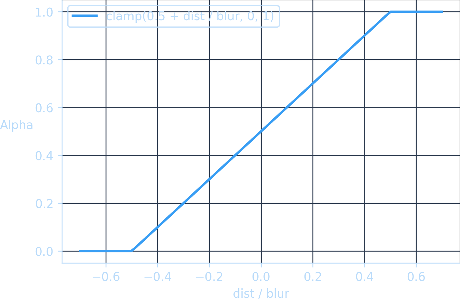
The harsh stops at
Loading canvas...
The smoothstep function can help here. Smoothstep is a family of interpolation functions that, as the name suggests, smooth the transition from
I’m defining smoothstep like so:
float smoothstep(float t) {return t * t * t * (t * (6.0 * t - 15.0) + 10.0);}
This is the “quintic” variant of the smoothstep function. It applies a bit more smoothing than the “default” smoothstep implementation.
Applying smoothstep to our alpha curve is quite simple:
float alpha = clamp(0.5 + dist / blur, 0.0, 1.0);alpha = smoothstep(alpha);
Below is a chart showing the smoothed alpha curve — I’ll include the original non-smoothed curve for comparison:
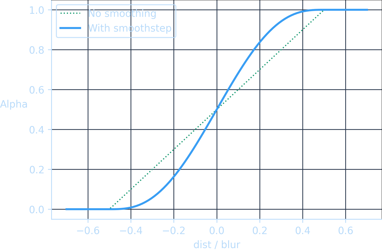
This results in a much smoother blur:
Loading canvas...
Following is a side-by-side comparison. The blur to the left is smoothed, while the right one is not.
Loading canvas...
That takes care of the sharp edges. Let’s now tackle the issue of the wave as a whole being too blurry.
Making the wave less uniformly blurry
Here’s our calc_blur method as we left it:
float calc_blur() {// ...float noise = simplex_noise(x * L + F * u_time, u_time * S);float t = (noise + 1.0) / 2.0;float blur = mix(1.0, BLUR_AMOUNT, t);return blur;}
The edge becomes sharper as
The canvas below has a visualization that illustrates this. The lower half is a chart showing the value of
Loading canvas...
You’ll notice that the wave becomes sharp when the chart gets close to touching the bottom — at values near zero — but it rarely dips that low. The value of
We can bias low values of
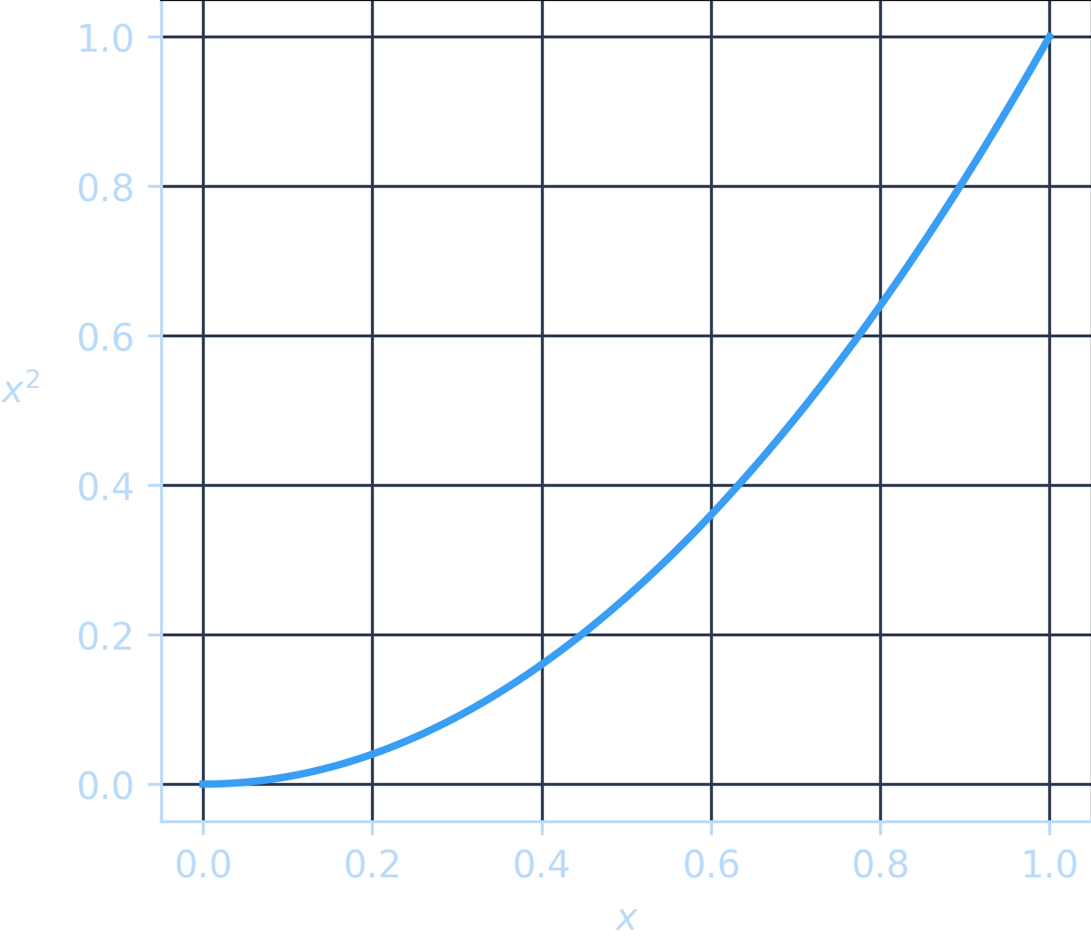
Consider how an exponent affects values between
The level of pull depends on the exponent. Here’s a chart of
This effect becomes more pronounced as we increase the exponent:
The following chart shows
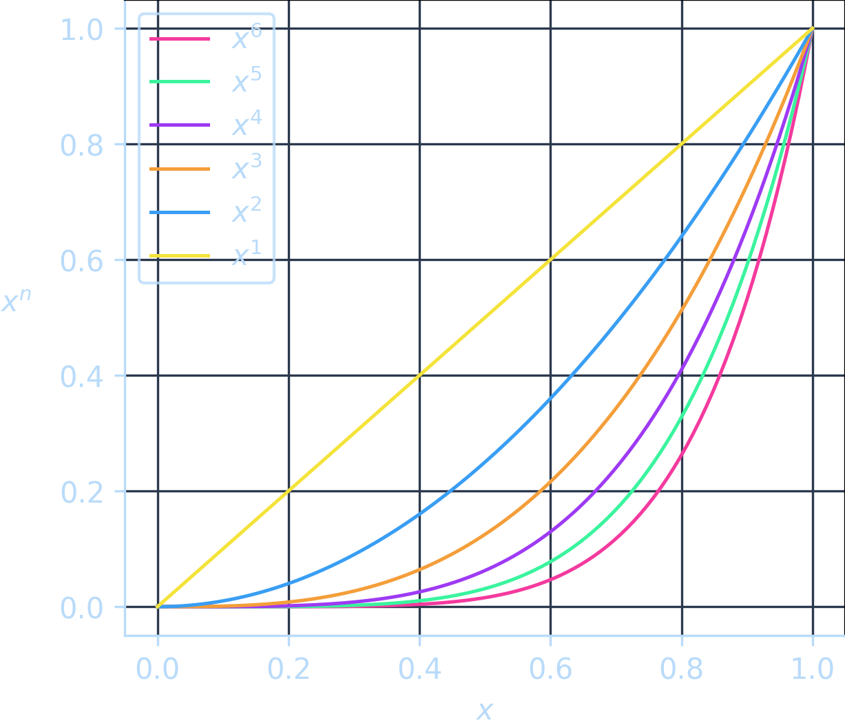
Notice how an exponent of
As you can see, a higher exponent translates to a stronger pull towards zero.
With that, let’s apply an exponent to pow function:
float t = (noise + 1.0) / 2.0;t = pow(t, exponent);
Below is a canvas that lets you vary the value of exponent from exponent to a default value of
Loading canvas...
As the exponent increases,
Let’s bring back the other wave and see what we’ve got:
Loading canvas...
Applying an exponent does dampen the strength of the blur, so let’s ramp the blur amount up — I’ll increase it from
Loading canvas...
Now we’re talking! We’ve got a pretty great-looking blur going!
Putting it all together
We’ve got all of the individual pieces we need to construct our final effect — let’s finally put it together!
Each wave is represented by an alpha value:
float w1_alpha = wave_alpha(WAVE1_Y, WAVE1_HEIGHT);float w2_alpha = wave_alpha(WAVE2_Y, WAVE2_HEIGHT);
We’re currently using those alpha values to blend three colors — these three shades of blue from the previous section:
vec3 bg_color = vec3(0.102, 0.208, 0.761);vec3 wave1_color = vec3(0.094, 0.502, 0.910);vec3 wave2_color = vec3(0.384, 0.827, 0.898);
The trick to our final effect lies in substituting each of those colors with a unique background noise and blending those.
We need our three background noises to be distinct. To support that we’ll update our background_noise function to take an offset value and add that to u_time. We’ve done this twice before so at this point this is just routine:
float background_noise(float offset) {float time = u_time + offset;float noise = 0.5;noise += simplex_noise(..., time * S) * ...;noise += simplex_noise(..., time * S) * ...;// ...return clamp(noise, 0.0, 1.0);}
We can now easily generate multiple distinct background noises. Let’s start by interpreting the background noises as lightness values:
float bg_lightness = background_noise(0.0);float w1_lightness = background_noise(200.0);float w2_lightness = background_noise(400.0);
We can blend these lightness values using the wave alpha values to calculate a final lightness value and pass vec3(lightness) to gl_FragColor:
float lightness = bg_lightness;lightness = mix(lightness, w1_lightness, w1_alpha);lightness = mix(lightness, w2_lightness, w2_alpha);gl_FragColor = vec4(vec3(lightness), 1.0);
This gives us the following effect:
Loading canvas...
Just try to tell me that this effect doesn’t look absolutely sick! It’s smooth, flowing, and quite dramatic at times.
The obvious next step is to map the final lightness value to a gradient. Let’s use this one:
Loading canvas...
Like before, we’ll get the texture into our shader via a uniform sampler2D:
uniform sampler2D u_gradient;
We then map the lightness value to the gradient like so:
gl_FragColor = texture2D(u_gradient, vec2(lightness, 0.5));
This applies the gradient to our effect:
Loading canvas...
Looks gorgeous. We can make this more sleek by increasing the height of the canvas a bit and adding a skew:
Loading canvas...
Sick, right? This could be used to add a modern and elegant touch to any landing page. Implementing the skew effect is deceptively simple — it’s just a transform of skewY(-6deg).
Since we’re generating the gradient in JavaScript, we can easily swap out the gradient. Here’s a canvas with a few cool gradients I picked:
Loading canvas...
It took a long time to get here, but we’ve ended up with something really cool.
Final words
I hope this was a good introduction to writing shaders, and I hope I provided you with the tools and intuition to get started writing shaders yourself!
At the beginning of the post I promised to link to the final shader code, so here it is.
The final shader includes a few additional elements that were not covered in the post. For example, the blur is calculated in multiple parts using an exponent range, adding a “haziness” element to the effect. I also added an oscillating “blur bias” to introduce periods of global blurriness and sharpness.
Take a look at this black-and-white version of the final effect and see if you can spot those elements (it’s much easier to see without color):
Loading canvas...
I didn’t cover these additional elements because they’re not core to the effect — they just add a layer of refinement. There are loads of ways in which you could tweak or add to the effect. I tried tons of ideas and kept those around because they worked very well. I suggest tweaking the code and trying to add some refinements yourself!
Huge thanks to my friends, Gunnlaugur Þór Briem and Eiríkur Fannar Torfason, for reading a draft version of this post — they provided great feedback.
Thanks so much for reading. Take what you learned and go write some awesome shaders!
— Alex Harri
To be notified of new posts, subscribe to my mailing list.